Summarise and analyse clinical trial information
Ralf Herold
2026-03-07
Source:vignettes/ctrdata_summarise.Rmd
ctrdata_summarise.RmdGeneral information on the ctrdata package is available
here: https://github.com/rfhb/ctrdata.
Remember to respect the registers’ terms and conditions (see
ctrOpenSearchPagesInBrowser(copyright = TRUE)). In any
publication, please cite this package as follows:
Herold R (2026). “Aggregating and analysing clinical trials data from
multiple public registers using R package ctrdata.” Research
Synthesis Methods, 17(3), 624-656. ISSN 1759-2879,
1759-2887. doi:10.1017/rsm.2025.10061 https://doi.org/10.1017/rsm.2025.10061. or
Herold R
(????). ctrdata: Retrieve and Analyze Clinical Trials Data from
Public Registers. R package version 1.26.1.9000, https://cran.r-project.org/package=ctrdata.
Preparations
Here using MongoDB, which may be faster than SQLite, can handle credentials, provides access to remote servers and can directly retrieve nested elements from paths. See Retrieve clinical trial information for examples using SQLite. Also PostgreSQL can be used as database, see Install R package ctrdata.
db <- nodbi::src_mongo(
  url = "mongodb://localhost",
  db = "my_database_name",
  collection = "my_collection_name"
)
db
# src: MongoDB
# ver: 8.0.10
# db(s): my_database_name
# size(s): 0 MB

# empty collection if exists
nodbi::docdb_delete(db, db$collection)
See Retrieve clinical trial information for more details.
# Load package
library(ctrdata)

# Model queries
queries <- ctrGenerateQueries(
  condition = "neuroblastoma",
  population = "P"
)

# Load trials from all queries into collection
result <- lapply(
  queries,
  ctrLoadQueryIntoDb,
  euctrresults = TRUE,
  euctrprotocolsall = FALSE,
  con = db)
# * Found search query from EUCTR: query=neuroblastoma&age=children&age=adolescent&age=infant-and-toddler&age=newborn&age=preterm-new-born-infants&age=under-18
# * Checking trials in EUCTR, found 106 trials
# - Downloading in 6 batch(es) (20 trials each; estimate: 7 s)...
# - Downloading 106 records of 106 trials (estimate: 5 s)...
# - Converting to NDJSON (estimate: 0.2 s)...
# - Importing records into database...
# = Imported or updated 106 records on 106 trial(s)
# * Checking results if available from EUCTR for 106 trials:
# - Downloading results...
# - Extracting results (. = data, F = file[s] and data, x = none): . F . . F .
# F . F . . F . . . . F . . F F . . . F . . . . . F . . F . F . . . . . F . . .
# . F . . F . .
# - Data found for 52 trials
# - Converting to NDJSON (estimate: 1 s)...
# - Importing 52 results into database (may take some time)...
# - Results history: not retrieved (euctrresultshistory = FALSE)
# = Imported or updated results for 52 trials
# No history found in expected format.
# Updated history ("meta-info" in "my_collection_name")
# * Found search query from ISRCTN: &q=&filters=condition:neuroblastoma,ageRange:Child,primaryStudyDesign:Interventional,phase:Phase 0,phase:Phase I,phase:Phase II,phase:Phase III,phase:Phase IV,phase:Phase I/II,phase:Phase II/III,phase:Phase III/IV
# * Checking trials in ISRCTN, found 1 trials
# - Downloading trial file (estimate: 0.03 s)...
# - Converting to NDJSON (estimate: 0.002 s)...
# - Importing records into database...
# = Imported or updated 1 trial(s)
# Updated history ("meta-info" in "my_collection_name")
# * Found search query from CTGOV2: cond=neuroblastoma&intr=Drug OR Biological&term=AREA[DesignPrimaryPurpose](DIAGNOSTIC OR PREVENTION OR TREATMENT)&aggFilters=ages:child,studyType:int
# * Checking trials in CTGOV2, found 474 trials
# - Downloading in 1 batch(es) (max. 1000 trials each; estimate: 1.3 s)...
# - Load and convert batch 1...
# - Importing records into database...
# JSON file #: 1 / 1
# = Imported or updated 474 trial(s)
# Updated history ("meta-info" in "my_collection_name")
# * Found search query from CTGOV2: term=AREA[ConditionSearch]"neuroblastoma" AND (AREA[StdAge]"CHILD") AND (AREA[StudyType]INTERVENTIONAL) AND (AREA[DesignPrimaryPurpose](DIAGNOSTIC OR PREVENTION OR TREATMENT)) AND (AREA[InterventionSearch](DRUG OR BIOLOGICAL))
# * Checking trials in CTGOV2, found 474 trials
# - Downloading in 1 batch(es) (max. 1000 trials each; estimate: 1.3 s)...
# - Load and convert batch 1...
# - Importing records into database...
# JSON file #: 1 / 1
# = Imported or updated 474 trial(s)
# Updated history ("meta-info" in "my_collection_name")
# * Found search query from CTIS: searchCriteria={"medicalCondition":"neuroblastoma","ageGroupCode":[2]}
# * Checking trials in CTIS, found 23 trials
# - Downloading and processing trial list (estimate: 0.9 s)...
# - Downloading and processing trial data (estimate: 6 s)...
# - Importing records into database...
# - Updating with additional data: .
# = Imported 23, updated 23 record(s) on 23 trial(s)
# Updated history ("meta-info" in "my_collection_name")

# Show results of loading
sapply(result, "[[", "n")
# EUCTR       ISRCTN       CTGOV2 CTGOV2expert         CTIS
#   106            1          474          474           23
Find fields / variables of interest
Specify a part of the name of a variable of interest; all variables
including deeply nested variable names are searched. Set
sample = TRUE (default) to rapidly execute the function in
large database collections. The search for fields is cached and thus
accelerated during the R session; calling
ctrLoadQueryIntoDb() or changing sample = ...
invalidates the cache.
# Find fields
dbFindFields(namepart = "date", sample = FALSE, con = db)
# Finding fields in database collection (may take some time) . . . . .
# Field names cached for this session.
# [...]
#                                                                       EUCTR
#                                    "n_date_of_competent_authority_decision"
# [...]
#                                                                      CTGOV2
# "annotationSection.annotationModule.unpostedAnnotation.unpostedEvents.date"
#                                                                      CTGOV2
#                       "protocolSection.statusModule.studyFirstSubmitQcDate"
# [...]
#                                                                        CTIS
#                                                               "publishDate"
#                                                                        CTIS
#                                                               "startDateEU"
# [...]
#                                                                      ISRCTN
#                                                "trialDesign.overallEndDate"
Data frame from database
The fields of interest can be obtained from the database and are represented in an R data frame, for example:
# Define vector of fields
fieldsOfInterest <- c(
  #
  # EUCTR protocol-related information
  "f41_in_the_member_state",
  "f422_in_the_whole_clinical_trial",
  "a1_member_state_concerned",
  #
  # EUCTR results-related information
  "trialInformation.recruitmentStartDate",
  "trialInformation.globalEndOfTrialDate",
  #
  # CTGOV2
  "protocolSection.statusModule.startDateStruct.date",
  "trialInformation.recruitmentStartDate",
  "protocolSection.statusModule.primaryCompletionDateStruct.date"
)

# Create data frame with records of trials
# which for at least one field have a value
result <- dbGetFieldsIntoDf(
  fields = fieldsOfInterest,
  con = db
)
# Querying database (7 fields)...

dim(result)
# [1] 567   8
Metadata from data frame
The objects returned by functions of this package include attributes with metadata to indicate from which database, table / collection and query details. Metadata can be reused in R.
attributes(result)
# [...]
#
# $class
# [1] "data.frame"
#
# $`ctrdata-dbname`
# [1] "my_database_name"
#
# $`ctrdata-table`  <-- this attribute will be retired by end 2024
# [1] "my_collection_name"
#
# $`ctrdata-table-note`
# [1] "^^^ attr ctrdata-table will be removed by end 2024"
#
# $`ctrdata-collection`
# [1] "my_collection_name"
#
# $`ctrdata-dbqueryhistory`
#       query-timestamp query-register query-records
# 1 2026-03-07 17:55:44          EUCTR           106
# 2 2026-03-07 17:55:45         ISRCTN             1
# 3 2026-03-07 17:55:47         CTGOV2           474
# 4 2026-03-07 17:55:50         CTGOV2           474
# 5 2026-03-07 17:55:53           CTIS            23
#query-term
# 1 query=neuroblastoma&age=children&age=adolescent&age=infant-and-toddler&age=newborn&age=preterm-new-born-infants&age=under-18
# 2 &q=&filters=condition:neuroblastoma,ageRange:Child,primaryStudyDesign:Interventional,phase:Phase 0,phase:Phase I,phase:Phase II,phase:Phase III,phase:Phase IV,phase:Phase I/II,phase:Phase II/III,phase:Phase III/IV
# 3 cond=neuroblastoma&intr=Drug OR Biological&term=AREA[DesignPrimaryPurpose](DIAGNOSTIC OR PREVENTION OR TREATMENT)&aggFilters=ages:child,studyType:int
# 4 term=AREA[ConditionSearch]"neuroblastoma" AND (AREA[StdAge]"CHILD") AND (AREA[StudyType]INTERVENTIONAL) AND (AREA[DesignPrimaryPurpose](DIAGNOSTIC OR PREVENTION OR TREATMENT)) AND (AREA[InterventionSearch](DRUG OR BIOLOGICAL))
# 5 searchCriteria={"medicalCondition":"neuroblastoma","ageGroupCode":[2]}
De-duplicate records
In the database, the variable “_id” is the unique index for a record. This “_id” is the NCT number for CTGOV records (e.g., “NCT00002560”), and it is the EudraCT number for EUCTR records including the postfix identifying the EU Member State (e.g., “2008-001436-12-NL”). It is relevant to de-duplicate records because a trial can be registered in both CTGOV2 and EUCTR, and can have records by involved country in EUCTR.
De-duplication is done at the analysis stage because this enables to
select if a trial record should be taken from one or the other register,
and from one or the other EU Member State. The basis of de-duplication
is the recording of additional trial identifiers in supplementary fields
(variables), which are checked and reported when using function
dbFindIdsUniqueTrials():
# Obtain de-duplicated trial record ids
ids <- dbFindIdsUniqueTrials(
  preferregister = "EUCTR",
  con = db
)
#Searching for duplicate trials...
# - Getting all trial identifiers (may take some time), 604 found in collection
# - Finding duplicates among registers' and sponsor ids...
# - Unique are 0 / 322 / 9 / 106 / 0 records from CTGOV / CTGOV2 / CTIS / EUCTR / ISRCTN
# = Returning keys (_id) of 437 records in collection "my_collection_name"

# Eliminate duplicate trials records:
result <- result[result[["_id"]] %in% ids, ]

nrow(result)
# [1] 422
#
# Note that "ids" are the identifiers of unique trials in the whole collection,
# whereas the data frame "result" only includes those trials in which any of
# the fields of interest had a value, thus explaining why "result" has fewer
# rows than "ids" has identifiers.
Use trial concepts to simplify analyses
An alternative is to calculate a column isUniqueTrial
already at the time that a data frame is created. This uses one of the
trial concepts that provide a canonical field, calculated from trial
information of any register, see
help(ctrdata-trial-concepts).
# Obtain data of interest
result <- dbGetFieldsIntoDf(
  fields = fieldsOfInterest,
  calculate = "f.isUniqueTrial",
  con = db
)
# To review trial concepts details, call 'help("ctrdata-trial-concepts")'
# Querying database (8 fields)...
# Searching for duplicate trials...
# - Getting all trial identifiers, 604 found in collection
# - Finding duplicates among registers' and sponsor ids...
# - Unique are 0 / 474 / 13 / 51 / 0 records from CTGOV / CTGOV2 / CTIS / EUCTR / ISRCTN
# = Returning keys (_id) of 538 records in collection "my_collection_name"

# Eliminate duplicate trials records:
result <- result[result[[".isUniqueTrial"]], ]

nrow(result)
# [1] 538
#
# Note this has used a different register as priority.
# Also, the data frame result includes all trials which
# had a value in at least one of the fields of interest
# or the fields needed to calculate the trial concept.

# See description of concept .isUniqueTrial:
help("f.isUniqueTrial")

# See how concept .isUniqueTrial is implemented
f.isUniqueTrial
Reviewing a specific trial
It will often be useful to inspect all data for a single trial, e.g. to understand the meaning and relation of fields, to see where certain information is stored, and to identify fields of interest.
For a given trial, function ctrShowOneTrial() enables the user to visualise the hiearchy of fields and contents in the user’s local web browser, to search for field names and field values, and to select and copy selected fields’ names for use with function dbGetFieldsIntoDf().
# Opens a web browser for user interaction.
# If the trial is not found in the database,
# it will be loaded from the register.
#
# The search is for both, field names and values
ctrShowOneTrial("2022-501725-21-00", con = db)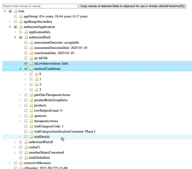 Alternatively, use any
standard database function to retrieve the trial’s
Alternatively, use any
standard database function to retrieve the trial’s JSON
representation that ctrdata had stored in the collection
and visualise its nested structure of field names and values.
# Requires additional package for visualisation
remotes::install_github("hrbrmstr/jsonview")

# Works with DuckDb, SQLite, PostgreSQL, MongoDB
oneTrial <- nodbi::docdb_query(
  src = db,
  key = db$collection,
  query = '{"_id":"2022-501725-21-00"}',
  limit = 1L
)

# Interactive widget where nodes can be expanded,
# note that fields and values cannot be searched
jsonview::json_tree_view(oneTrial)
Simple analysis of dates
In a data frame generated with dbGetFieldsIntoDf(),
fields are typed as dates, logical, character or numbers. This typing
facilitates using the data for analysis, for example of dates with base
R graphics:
# Get data of interest
result <- dbGetFieldsIntoDf(
  fields = "ctrname",
  calculate = c("f.isUniqueTrial", "f.startDate"),
  con = db
)

str(result)
# 'data.frame': 604 obs. of  4 variables:
#  $ _id           : chr  "2004-004386-15-ES" "2005-000915-80-IT" "2005-001267-63-IT" ...
#  $ ctrname       : chr  "EUCTR" "EUCTR" "EUCTR" "EUCTR" ...
#  $ .isUniqueTrial: logi  FALSE FALSE FALSE FALSE TRUE TRUE ...
#  $ .startDate    : Date, format: "2005-11-15" "2005-04-21" "2005-07-08" ...

# Open file for saving
png("vignettes/nb1.png")

# De-duplicate and visualise start date
hist(
  result[result$.isUniqueTrial, ".startDate"],
  breaks = "years"
)
box()
dev.off()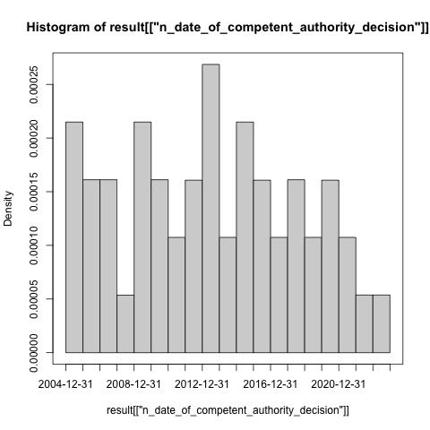
Cross-register clinical trial concepts
A number of calculations across fields from different registers are
available in ctrdata. This offers much convenience for
users, because it provides a canonical understanding and implementation
of the mapping of corresponding fields and value lists across different
registers. Available calculations can be listed, and a specific
documentation shown.
# Introduction and overview of available trial concepts
help("ctrdata-trial-concepts")

# Show documentation of a specific trial concept
help("f.isMedIntervTrial")

# List concepts available at this time
as.character(utils::ls.str(
  getNamespace("ctrdata"),
  all.names = TRUE,
  pattern = "^f[.][a-z]"))
#  [1] "f.assignmentType"             "f.controlType"                "f.externalLinks"
#  [4] "f.hasResults"                 "f.isMedIntervTrial"           "f.isUniqueTrial"
#  [7] "f.likelyPlatformTrial"        "f.numSites"                   "f.numTestArmsSubstances"
# [10] "f.primaryEndpointDescription" "f.primaryEndpointResults"     "f.resultsDate"
# [13] "f.sampleSize"                 "f.sponsorType"                "f.startDate"
# [16] "f.statusRecruitment"          "f.trialObjectives"            "f.trialPhase"
# [19] "f.trialPopulation"            "f.trialTitle"
Merging fields for analysis
With the function dfMergeVariablesRelevel(), users have
control how to merge values of a set of original variables to a new
variable, optionally with a new set of values. For more, see
help(dfMergeVariablesRelevel). This can be used for
concepts that are very specific to the use case and / or not implemented
so far, see help(ctrdata-trial-concepts).
Historic versions of trial records and changes in sample sizes
Historic versions can set to be retrieved for CTGOV2 by specifying
ctgov2history = <...> when using
ctrLoadQueryIntoDb(); this functionality was added in
ctrdata version 1.18.0. The versions include all trial data
available at the date of the respective version. Only CTGOV2 provides
historic versions at this time (CTIS only until its relaunch on
2024-06-17) as part of their respective APIs.
Nevertheless, historic versions can also be created for CTIS by
specifying querytoupdate = <...>, ctishistory = TRUE
when using ctrLoadQueryIntoDb(); this functionality thus is
not provided by the register but triggered by the user, it was added in
ctrdata version 1.21.1.9000.
The following schema represents two clinical trial records (one each
from CTGOV2 and CTIS) with the array of history: [...]
versions as part of a trial’s record (the ellipsis ...
represents all other data fields):
'
[
  {
   "_id":"NCT01234567",
   "title": "Current title",
   "clinical_results": ...,
   ...,
   "history": [
     {
      "history_version": {
        "version_number": 1,
        "version_date": "2020-21-22 10:11:12"},
      "title": "Original title",
      "clinical_results": ...,
      ...
     },
     {
      "history_version": {
        "version_number": 2,
        "version_date": "2021-22-23 11:13:13"},
      "title": "Later title",
      "clinical_results": ...,
      ...
     }
   ]
  },
  {
   "_id":"2022-502051-56-00",
   "title": "Current title",
   "ctrname": "CTIS",
   "lastUpdated": "2025-04-07"
   "authorizedPartsII": ...,
   ...,
   "history": [
     {
      "history_version": {
        "version_number": 0,
        "version_date": "2025-04-06"},
      "title": "Intermediate title",
      "ctrname": "CTIS",
      "lastUpdated": "2025-04-06"
      "authorizedPartsII": ...,
      ...
     },
     {
      "history_version": {
        "version_number": 0,
        "version_date": "2025-04-05"},
      "title": "Original title",
      "ctrname": "CTIS",
      "lastUpdated": "2025-04-05"
      "authorizedPartsII": ...,
      ...
     }
   ]
  },
  ...
]
'
The example shows how planned or realised number of participants (sample size) changed over time for individual trials, using available data
# Load previous query (above), specifying that
# for each trial, 5 versions should be retrieved
ctrLoadQueryIntoDb(
  queryterm = queries["CTGOV2"],
  con = db,
  ctgov2history = 5L
)
# * Found search query from CTGOV2: cond=neuroblastoma&intr=Drug OR Biological&term=AREA[DesignPrimaryPurpose](DIAGNOSTIC OR PREVENTION OR TREATMENT)&aggFilters=ages:child,studyType:int
# * Checking trials in CTGOV2, found 474 trials
# - Downloading in 1 batch(es) (max. 1000 trials each; estimate: 1.3 s)...
# - Load and convert batch 1...
# - Importing records into database...
# JSON file #: 1 / 1
# * Checking and processing historic versions (estimate: 24 s)...
# - Downloading 2173 historic versions (estimate: 109 s)...
# - Merging trial versions . . . . . . . . . . . . . . . . . . . . . . . . . .
# - Updating trial records . . . . . . . . . . . . . . . . . . . . . . . . . .
# Updated 474 trial(s) with historic versions
# = Imported or updated 474 trial(s)
# Updated history ("meta-info" in "my_collection_name")
# $n
# [1] 474

# Get relevant fields
result <- dbGetFieldsIntoDf(
  fields = c(
    # use CTGOV2 structured historic information
    "history.history_version.version_date",
    "history.protocolSection.designModule.enrollmentInfo.count"
  ),
  calculate = "f.statusRecruitment",
  con = db
)

# Helper packages
library(dplyr)
library(tidyr)
library(ggplot2)

# Mangle and plot
result %>%
  unnest(cols = starts_with("history.")) %>%
  filter(.statusRecruitment == "completed") %>%
  filter(!is.na(history.protocolSection.designModule.enrollmentInfo.count)) %>%
  filter(history.protocolSection.designModule.enrollmentInfo.count > 0L) %>%
  group_by(`_id`) %>%
  ggplot(
    mapping = aes(
      x = history.history_version.version_date,
      y = history.protocolSection.designModule.enrollmentInfo.count,
      colour = `_id`)
  ) +
  geom_step() +
  geom_point() +
  theme_light() +
  scale_y_log10() +
  guides(colour = "none") +
  labs(
    title = "Sample sizes in trials including patients with a neuroblastoma",
    subtitle = "Source: CTGOV2 records labelled as phase 3 and completed",
    caption = Sys.Date()
  )

ggsave("vignettes/samplesizechanges.png", width = 6, height = 4)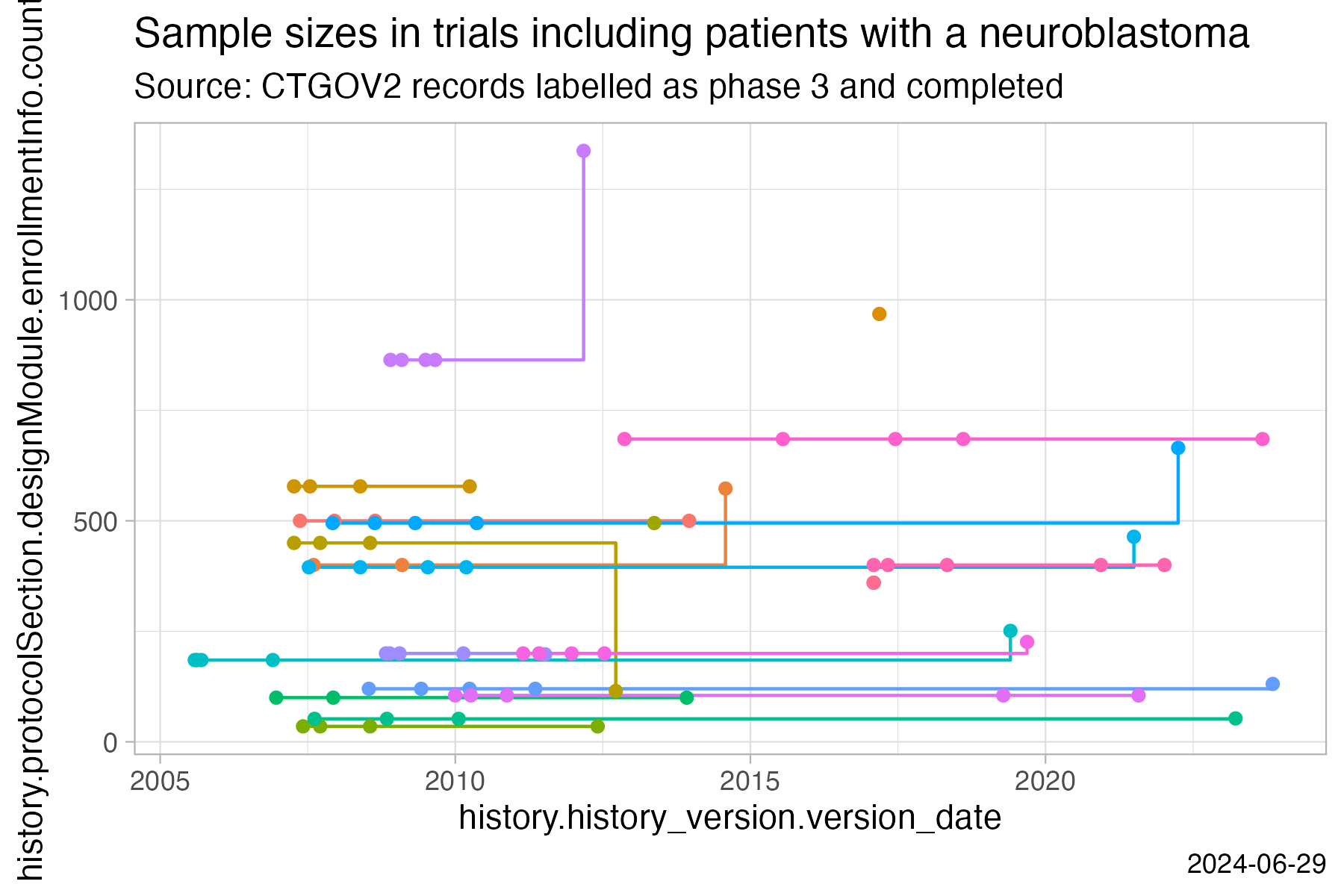
Analysing nested fields such as trial results
The registers represent clinical trial information by nesting fields (e.g., several reporting groups within several measures within one of several endpoints). A visualisation of this hierarchical representation for CTGOV2 follows. Compare this with the outcome measures presented here: https://clinicaltrials.gov/study/NCT02139397?tab=results#outcome-measures, specifically “3. Determine the Progression Free Survival (PFS)…”
# Since version 1.20.0, an interactive widget is built into ctrdata
# and can be used to search in all field names and all values
ctrShowOneTrial("NCT02139397", con = db)
See example for ctrShowOneTrial() in section Reviewing a specific trial. An
alternative is:
# Helper package
remotes::install_github("https://github.com/hrbrmstr/jsonview")

# Get relevant data
result <- dbGetFieldsIntoDf("resultsSection.outcomeMeasuresModule", con = db)

# Create interactive widget
jsonview::json_tree_view(result[result[["_id"]] == "NCT02139397", -1])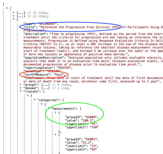
The analysis of nested information such as the highlighted duration
of response is facilitated with ctrdata as follows. The
main steps are:
Create a data from fields identified as shown in previous sections (using
dbGetFieldsIntoDf())Transform nested information to a long, name-value data frame (using
dfTrials2Long())Identify the measures of interest (e.g. PFS, blue circle above) by specifying the name and value of these fields (
wherename,wherevaluein functiondfName2Value())Obtain values by specifying the name(s) of its value field(s) (red and green circles in figure above;
valuenamein functiondfName2Value())Tabulate the results of interest
This is put together in the following example. Note that
CTGOV fields are no longer downloadable (see NEWS.md) but
may exist in previously created databases.
#### 1. Create data frame from results fields
# These are key results fields from
# CTGOV2, CTGOV and from EUCTR:
result <- dbGetFieldsIntoDf(
  fields = c(
    # EUCTR - note this requires to set parameter
    # euctrresults = TRUE in ctrLoadQueryIntoDb()
    # as shown above in section "User annotations"
    "trialInformation.populationAgeGroup",
    "subjectDisposition.recruitmentDetails",
    "baselineCharacteristics.baselineReportingGroups.baselineReportingGroup",
    "endPoints.endPoint",
    "subjectAnalysisSets",
    "adverseEvents.seriousAdverseEvents.seriousAdverseEvent",
    # CTGOV2
    "resultsSection.outcomeMeasuresModule",
    "protocolSection.designModule.designInfo.allocation",
    "resultsSection.participantFlowModule",
    # CTGOV
    "clinical_results.baseline.analyzed_list.analyzed.count_list.count",
    "clinical_results.baseline.group_list.group",
    "clinical_results.baseline.analyzed_list.analyzed.units",
    "clinical_results.outcome_list.outcome",
    "study_design_info.allocation"
  ),
  calculate = "f.isUniqueTrial",
  con = db
)

# Keep only unique trial records
result <- result[result[[".isUniqueTrial"]], ]


#### 2. All nested data are transformed to a long,
# Name value data frame (which has several hundred
# rows for each trial, with one row per field):
#
long_result <- dfTrials2Long(df = result)
# Total 98225 rows, 160 unique names of variables
long_result[c(100, 10000, 80000), ]
# # A tibble: 3 × 4
#   `_id`             identifier name                                                                 value
#   <chr>             <chr>      <chr>                                                                <chr>
# 1 2007-000371-42-DE 36         adverseEvents.seriousAdverseEvents.seriousAdverseEvent.dictionaryOv… false
# 2 2013-000885-13-FR 92         adverseEvents.seriousAdverseEvents.seriousAdverseEvent.dictionaryOv… false
# 3 NCT01767194       1.2        resultsSection.outcomeMeasuresModule.outcomeMeasures.denoms.counts.… 17

#### 3. and 4. Obtain values for measures of interest
#
# The parameters can be regular expressions
clinicalDuration <- dfName2Value(
  df = long_result,
  # 3. Identify measures of interest
  wherename = paste0(
    "endPoints.endPoint.title|",
    "resultsSection.outcomeMeasuresModule.outcomeMeasures.title"
  ),
  wherevalue = paste0(
    "duration of response|DOR|",
    "free survival|DFS|PFS|EFS"
  ),
  # 4. Obtain result values for measure
  valuename = paste0(
    "resultsSection.*outcomeMeasures.classes.categories.measurements.value|",
    "endPoints.*armReportingGroup.tendencyValues.tendencyValue.value|",
    "resultsSection.outcomeMeasuresModule.outcomeMeasures.unitOfMeasure|",
    "endPoints.endPoint.unit|",
    "resultsSection.outcomeMeasuresModule.outcomeMeasures.groups.title|",
    "endPoints.*armReportingGroup.armId"
  )
)
# Returning values for 61 out of 538 trials


#### 5. Tabulate the results

# PFS / EFS duration has been reported with various units:
sort(unique(clinicalDuration[
  grepl("unit", clinicalDuration$name), "value", drop = TRUE]))
#  [1] "3 year EFS"                               "Days"
#  [3] "Estimated probability"                    "L/hr"
#  [5] "months"                                   "Months"
#  [7] "number of participants with No VOD/Death" "Participants"
#  [9] "percent of probability"                   "percent probability"
# [11] "Percent Probability"                      "percentage"
# [13] "Percentage"                               "percentage of 3 yr EFS survival"
# [15] "percentage of participants"               "Percentage of participants"
# [17] "percentage of participent"                "Percentage of patients"
# [19] "percentage of subjects without an event"  "Percentage probability"
# [21] "Probability"                              "Proportion of participants"
# [23] "weeks"                                    "Weeks"

# Helper packages for convenience
library(dplyr)
library(tidyr)

# Mangle data for tabulation
clinicalDuration %>%
  as_tibble() %>%
  mutate(
    group_id = paste0(`_id`, "_", sub("([0-9]+)[.]?.*", "\\1", identifier)),
    name_short = sub(".*[.](.+)", "\\1", name),
    name_short = if_else(name_short == "unitOfMeasure", "unit", name_short)
  ) %>%
  group_by(group_id) %>%
  mutate(
    is_duration = any(grepl("day|month|week|year", value, ignore.case = TRUE))) %>%
  ungroup() %>%
  filter(is_duration) %>%
  select(name_short, value, where, group_id) %>%
  pivot_wider(id_cols = c(group_id, where), names_from = name_short, values_fn = list) %>%
  unnest(c(value, unit)) %>%
  filter(!grepl("999[9]*", value)) %>%
  rowwise() %>%
  mutate(
    value = as.numeric(value),
    arm_names = paste(armId, title, collapse = " / ")
  ) %>%
  ungroup() %>%
  mutate(
    days = case_when(
      grepl("[wW]eek", unit) ~ value * 7,
      grepl("[mM]onth", unit) ~ value * 30,
      grepl("[yY]ear", unit) ~ value * 30,
      .default = value
    )) %>%
  select(!c(value, unit, armId, title)) -> clinicalDuration

clinicalDuration[sample(seq_len(nrow(clinicalDuration)), 10L), ]
# # A tibble: 10 × 4
#    group_id             where                                                             arm_names  days
#    <chr>                <chr>                                                             <chr>     <dbl>
#  1 NCT00867568_4        Progression Free Survival (PFS) of Participants Using Days From … " TPI 28…  186
#  2 2013-003595-12-ES_3  Progression Free Survival (PFS) as assessed by the Investigator … "Arm-115…  162
#  3 2014-004685-25-ES_14 DOR as Determined by the Investigator RANO criteria for Particip… ""          NA
#  4 2014-004685-25-ES_10 PFS as Determined by the Investigator using RECIST v1.1 criteria… ""          NA
#  5 NCT01587703_53       Progression Free Survival-Part 1 BID                              " Part 1…  240
#  6 2014-004697-41-ES_17 DOR as Determined by the Investigator Using mINRC in Participant… "Arm-104…   NA
#  7 NCT01125800_8        Duration of Response by Treatment                                 " Pediat…  146.
#  8 NCT01742286_3        Duration of Response (DoR) Per Investigator Assessment            " ALK-ac…   NA
#  9 NCT04029688_15       Part 1b: PFS in Participants With TP53 WT Neuroblastoma Assessed… " Part 1…   51
# 10 2014-004685-25-ES_11 PFS as Determined by the Investigator using RANO criteria for Pa… ""          NA
Analysing primary endpoints
Text analysis has to be used for many fields of trial information
from the registers. Here is an example to simply categorise the type of
primary endpoint. In addition, the number of subjects are compared by
type of primary endpoint. The example uses trial concepts introduced in
earlier sections, see help(ctrdata-trial-concepts).
# Get relevant data
result <- dbGetFieldsIntoDf(
  calculate = c(
    "f.isUniqueTrial",
    "f.sampleSize",
    "f.trialPopulation",
    "f.primaryEndpointDescription"
  ),
  con = db
)

# De-duplicate
result <- result[result[[".isUniqueTrial"]], ]

# For primary endpoint of interest, use regular expression on text to
# identify time to the respective event (mostly includes death events)
regex <- "((progression|event|relapse|recurrence|disease)[- ]free)|pfs|dfs|efs)"

# .primaryEndpointDescription is in each cell a list of one or more
# items with an endpoint description; grepl works on each such item
result$pep_is_efs <- grepl(
  pattern = regex,
  x = result$.primaryEndpointDescription,
  ignore.case = TRUE
)

# Tabulate
table(result$pep_is_efs)
# FALSE  TRUE
#   471    67

# Plot
library(ggplot2)
ggplot(
  data = result,
  aes(
    x = .sampleSize,
    y = pep_is_efs
  )
) +
  geom_boxplot() +
  scale_x_log10()

ggsave("vignettes/boxpep.png", width = 6, height = 4)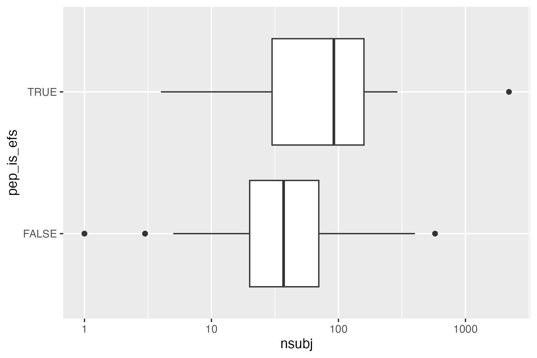
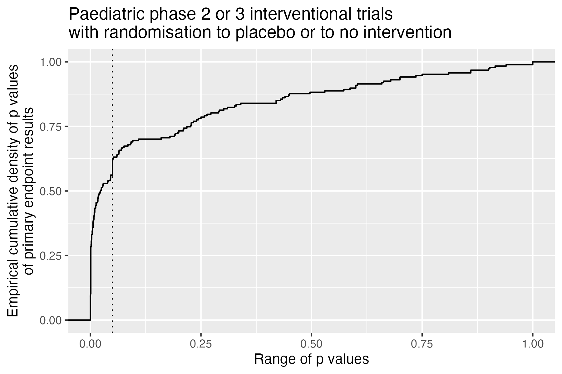
Analysis methods and p values
It may be interesting to review results of the primary endpoint in a set of trials, for a therapeutic area or a types of endpoints or designs. The results of null-hypothesis significance testing (NHST) may show an interesting distribution of p values (see also Robinson-D 2014, http://varianceexplained.org/statistics/interpreting-pvalue-histogram/, which refers to cases with many p values, possibly from a single experiment). When analysed robustly in a well-defined set of trials, such distributions may allow assumptions about equipoise, forking path or reporting preferences.
The example merely shows the technical approach, without asserting
relevance. For a robust analysis, consider further trial concepts (in
particular, “f.trialObjectives”, “f.controlType”, “f.isMedIntervTrial”,
“f.trialPhase”), see help(ctrdata-trial-concepts).
# Get result set
result <- dbGetFieldsIntoDf(
calculate = c(
"f.isUniqueTrial",
"f.sampleSize",
"f.primaryEndpointResults"
),
con = db
)
# De-duplicate
result <- result[result[[".isUniqueTrial"]], ]
# Helper package
library(ggplot2)
# Plot p values ECDF
ggplot(
data = result,
aes(x = .primaryEndpointFirstPvalue)) +
stat_ecdf(geom = "step") +
labs(
title = "Trials with children with a neuroblastoma",
x = "Range of p values",
y = "Empirical cumulative density of p values\nfrom primary endpoint primary analysis") +
geom_vline(
xintercept = 0.05,
linetype = 3)
ggsave("vignettes/phase23_paed_p_values.png", width = 6, height = 4)
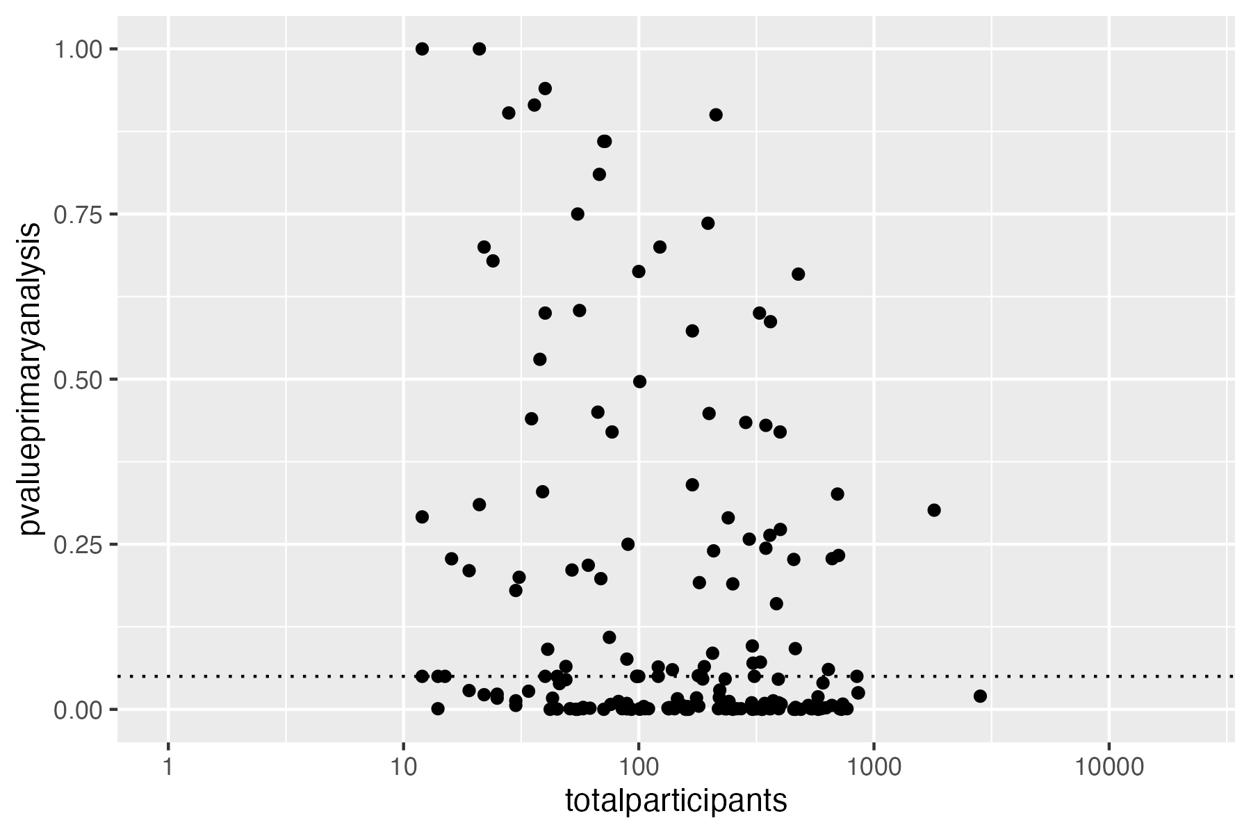
# Plot sample size vs. p value
ggplot(
data = result,
aes(
x = .sampleSize,
y = .primaryEndpointFirstPvalue)) +
geom_point() +
ylim(0, 1) +
xlim(0, 1000) +
scale_x_log10() +
geom_hline(yintercept = 0.05, linetype = 3)
ggsave("vignettes/phase23_paed_p_values_participants.png", width = 6, height = 4)
# Statistical method used for primary endpoint analysis
tmp <- table(result$.primaryEndpointFirstPmethod)
tmp <- tmp[rev(order(tmp))]
tmp <- data.frame(tmp)
knitr::kable(tmp)| Var1 | Freq |
|---|---|
| logrank | 3 |
| fisherexact | 2 |
| wilcoxon | 1 |
| ttest2sided | 1 |
| regressioncox | 1 |
| exactonesidedbinomialtest | 1 |
| chisquared | 1 |
Investigational or authorised medicinal product?
The information about the status of authorisation (licensing) of a
medicine used in a trial is recorded in EUCTR in the field
dimp.d21_imp_to_be_used_in_the_trial_has_a_marketing_authorisation.
A corresponding field in CTGOV, CTGOV2 and ISRCTN is not known. The
status is in the tree starting from the dimp element.
# Helper package
library(dplyr)

# Get results
result <- dbGetFieldsIntoDf(
  fields = c(
    "a1_member_state_concerned",
    "n_date_of_competent_authority_decision",
    "dimp.d21_imp_to_be_used_in_the_trial_has_a_marketing_authorisation",
    "x6_date_on_which_this_record_was_first_entered_in_the_eudract_database",
    "f422_in_the_whole_clinical_trial",
    "a2_eudract_number"
  ),
  calculate = c(
    "f.isUniqueTrial",
    "f.startDate"
    ),
  con = db
) %>%
  filter(.isUniqueTrial)

# How many of the investigational medicinal product(s)
# that are being used in the trial are authorised?
number_authorised <- sapply(
  result[["dimp.d21_imp_to_be_used_in_the_trial_has_a_marketing_authorisation"]],
  function(i) if (all(is.na(i))) NA else sum(i, na.rm = TRUE)
)
table(number_authorised, exclude = "")
# number_authorised
#    0    1    2    3    4    5    7 <NA>
#   19   12    7    4    2    3    1  490

result[["any_authorised"]] <- number_authorised > 0L

# Helper packages
library(ggplot2)
library(scales)
library(dplyr)

# Plot
ggplot(
  data = result %>%
    filter(!is.na(any_authorised)),
  aes(
    x = .startDate,
    fill = any_authorised
  )
) +
  scale_x_date(
    breaks = breaks_width(width = "2 years"),
    labels = date_format("%Y")
  ) +
  geom_histogram(binwidth = 2 * 365.25) +
  labs(
    title = "Selected clinical trials in EU",
    x = "Year of trial start",
    y = "Number of trials",
    fill = "Medicine\nauthorised?"
  )

ggsave("vignettes/nbtrials.png", width = 6, height = 4)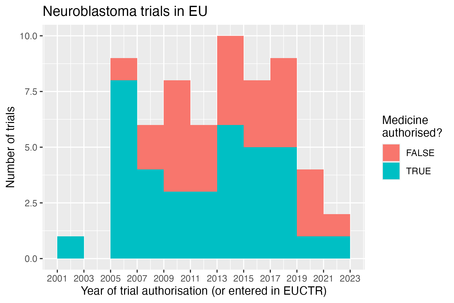
Analyses using MongoDB pipeline
Here is an example of analysis functions that can be run directly on a MongoDB server, which are fast and do not consume R resources.
# Load package for database access
library(mongolite)

# Create R object m to access the
# collection db created above
m <- mongo(
  url = paste0(db[["url"]], "/", db[["db"]]),
  collection = db[["collection"]]
)

# Number of records in  collection
m$count()
# [1] 605

# Number of EUCTR records, using JSON for query
m$count(query = '{"_id": {"$regex": "[0-9]{4}-[0-9]{6}-[0-9]{2}-[3A-Z]{2,3}", "$options": "i"}}')
# [1] 106

# Alternative
m$count(query = '{"ctrname": "EUCTR"}')
# [1] 106

# Number of CTGOV records
m$count(query = '{"_id": {"$regex": "NCT[0-9]{8}", "$options": "i"}}')
# [1] 474

# Alternative
m$count(query = '{"ctrname": "CTGOV2"}')
# [1] 474

# To best define regular expressions for analyses, inspect the field:
head(
  m$distinct(
    key = "protocolSection.outcomesModule.primaryOutcomes.measure",
    query = '{"ctrname": "CTGOV2"}'
  )
)
# [1] "- To demonstrate that 123I-mIBG planar scintigraphy is ...
# [2] "1-year Progression-free Survival"
# [3] "18F-mFBG PET Scan identification of Neuroblastoma on the LAFOV PET/CT"
# [4] "2-year progression free survival"
# [5] "2-year progression free survival (PFS)"
# [6] "AE"
Aggregation
The following example uses the aggregation pipeline in MongoDB. See here for details on mongo’s aggregation pipleline: https://www.mongodb.com/docs/manual/core/aggregation-pipeline/
#
# Total count of PFS, EFS, RFS or DFS
out <- m$aggregate(
  # Count number of documents in collection that
  # matches in primary_outcome.measure the
  # regular expression,
  pipeline =
    '[{"$match": {"protocolSection.outcomesModule.primaryOutcomes.measure":
      {"$regex": "(progression|event|relapse|recurrence|disease)[- ]free",
                 "$options": "i"}}},
      {"$group": {"_id": "null", "count": {"$sum": 1}}}]'
)
out
#    _id count
# 1 null    56

# List records of trials with overall survival
# as primary endpoint, and list start date
out <- m$aggregate(
  pipeline =
    '[{"$match": {"protocolSection.outcomesModule.primaryOutcomes.measure":
      {"$regex": "overall survival", "$options": "i"}}},
      {"$project": {"_id": 1, "protocolSection.statusModule.startDateStruct.date": 1}}]'
)
head(out)
#           _id       date
# 1 NCT00793845    2008-08
# 2 NCT05303727    2022-08
# 3 NCT00923351 2007-06-02
# 4 NCT03275402 2018-12-11
# 5 NCT04897880 2019-01-09
# 6 NCT00637637    2007-09
Mapreduce
Since Mapreduce is deprecated since MongoDB version 5 (https://www.mongodb.com/docs/manual/core/map-reduce/), use an aggregation pipeline:
# Count number of trials by number of study
# participants in bins of hundreds of participants:
m$aggregate(pipeline = '
[{"$project": {
    "flooredNumber": {
      "$multiply": [
        { "$floor": {
            "$divide": [
               { "$toInt": "$protocolSection.designModule.enrollmentInfo.count"},
                100 ] } },
          100] } } },
  { "$group": {
      "_id": "$flooredNumber",
      "count": { "$count": {} } } },
  { "$sort": { "_id": 1 } }
]
')
#     _id count
# 1    NA   157
# 2     0   364
# 3   100    49
# 4   200    11
# 5   300     4
# 6   400     6
# 7   500     4
# 8   600     4
# 9   700     1
# 10  800     2
# 11  900     1
# 12 1400     1
# 13 3300     1